Behind the Assumptions
The simulator takes parameters as given. This section asks what happens when they're not.
If you only have a few minutes
This section is long. The short version: the Markowitz portfolio optimization framework produces precise-looking “optimal” allocations, but the precision is largely illusory. When you account for realistic uncertainty in the inputs (Chapter 2), drift in those inputs over time (Chapter 3), and the compounding effects of more than two assets (Chapter 4), the “optimal” portfolio dissolves into a wide cloud of equally-defensible answers, and the cloud is moving from era to era.
This isn’t a flaw in the math — it’s a feature of the gap between the framework’s clean assumptions and the messy world it’s applied to.
The interactive widgets in Chapters 1, 2, and 4 are the centerpiece of this section. If you don’t read anything else, scroll through and play with those.
Bottom line (Chapter 4’s closing reflection): the framework is genuinely useful as a thinking aid — it sharpens intuition about diversification and risk-return tradeoffs — but its specific numerical outputs shouldn’t be taken as recommendations. They’re a single point in a cloud of plausible answers, all drifting over time.
The Monte Carlo simulator on the main page asks a specific question: given fixed assumptions about expected returns, volatilities, and correlations, what’s the distribution of outcomes you might experience? That’s a useful question, and the simulator’s answer — distributions, not point estimates — is more honest than the standard textbook treatment.
But the question itself assumes a lot. It assumes the parameters are settled. It assumes they stay the same over your investment horizon. It assumes the framework you’re using to compute “optimal” portfolios is reliable when fed those parameters. None of those assumptions are obviously true in the real world.
This section steps back one layer in the chain of assumptions. Each chapter takes one piece of the framework that the simulator treated as given and asks: what if it isn’t?
Two ways to think about uncertainty
Before the chapters begin, it’s worth being clear about what kind of uncertainty this section is examining, because there’s another kind — addressed by the main simulator on the home page — that’s easy to conflate with it.
The Monte Carlo simulator shows that even with a single set of input parameters, outcomes are uncertain. A 60/40 portfolio over a specific period doesn’t produce one expected return; it produces a distribution of possible returns. The textbook frontier curve summarizes this distribution as a single point (its mean), but the cloud is still there, hiding behind the point. (The curve is actually a series of these points, one for each possible allocation — each point along the curve is itself a summary of a cloud like the one shown below.)
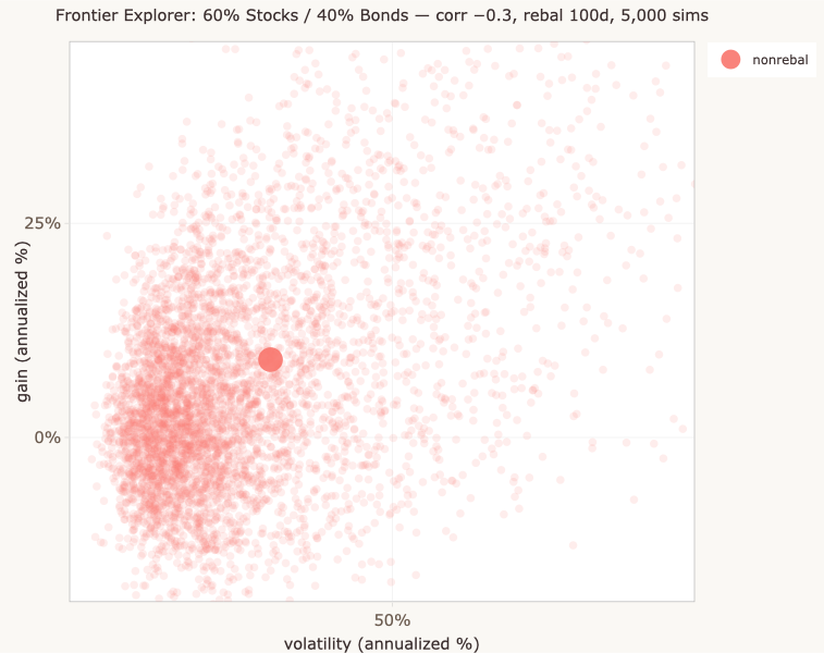
The simulator could be elaborated in many ways — for example, by letting parameters evolve over time within each run rather than holding them constant. But these elaborations don’t address the deeper question of what parameter values to start from in the first place.
This section examines that deeper question. Even with a single set of parameter values fully specifying a generative process, we have to ask what values to use — and reasonable analysts would pick differently. Propagating this uncertainty means running the analysis across many plausible combinations of values and looking at the combined distribution of answers, not just the answer from one combination.
The animation below shows the contrast. On the left: a single parameter set drives one generative process, producing a distribution of outcomes — what the main simulator does. On the right: a distribution of parameter sets, each driving its own generative process, producing a wider combined distribution — what this section’s chapters are about. The combined distribution is honest about both the within-run variation and the across-set variation; the simulator’s single-set version is honest about only one.
A note on the cartoon’s simplicity. The animation uses a single parameter (a probability) for visual clarity. Real generative models — including the main simulator — use several parameters at once (expected returns, volatilities, correlations). The same logic applies: a single set of parameter values produces one distribution of outcomes; many sets produce a combined distribution. The cartoon’s pipeline shape generalizes to any number of parameters; the visual just gets harder to draw.
Two ways to think about uncertainty
What changes when you acknowledge parameter uncertainty
Inspired by Figure 3.6 in Richard McElreath’s Statistical Rethinking (2nd ed.).
Fixed parameter
A single parameter value produces a distribution of outcomes. This is what a standard Monte Carlo simulator does — fixed parameters, distribution of outcomes. The simulator is honest about outcome uncertainty: given exactly these parameters, here’s the range of possible histories.
Uncertain parameter
A distribution over parameter values propagates through to a wider distribution of outcomes. Each parameter value contributes its own sampling distribution, weighted by how plausible the parameter value is. The combined distribution at the bottom is wider than any single parameter’s contribution.
The parameter uncertainty widgets on this page do part of the uncertain-parameter approach — they show the cloud of summary statistics (optimal allocations, Sharpe ratios) that comes from varying parameters. They don’t combine that with the full sampling distributions for each parameter set, which would yield the full combined outcome distribution shown on the right. The cartoon shows what that full picture would look like in principle.
The structural point: relying on a single point estimate of a parameter — even if you correctly propagate outcome uncertainty given that estimate — produces an overconfident distribution.
McElreath calls this “the illusion of certainty that arises from tossing away uncertainty about the parameters.”
What does ‘optimal’ mean?
Before we can examine the framework, we have to know what it’s claiming. This chapter introduces the Sharpe ratio and the tangency portfolio — the standard way of comparing portfolios that differ in both expected return and risk, and the standard definition of “optimal” that falls out of that comparison.
→ Read Chapter 1How much does the answer depend on the inputs?
The framework gives precise-looking answers, but those answers depend on input parameters that come with real uncertainty. Even modest variation in those inputs produces wide variation in what the framework calls “optimal.” This chapter shows what happens when you propagate parameter uncertainty through the optimization: the precise-looking answer becomes a cloud of equally-defensible answers.
→ Read Chapter 2When parameters drift
The inputs to portfolio optimization are typically derived from historical data — what stocks averaged over the past few decades, how volatile bonds were, how the two moved together. But the historical summaries themselves shift over time. A historical chart of stock-bond correlation makes this concrete: it isn’t a number that holds steady; it takes different values in different eras, sometimes shifting sharply enough to flip sign.
→ Read Chapter 3Three assets and beyond
With only two assets, “optimization” is trivial — every allocation is uniquely determined by the stock-bond split. With three or more assets, optimization becomes a real choice, and parameter uncertainty compounds. The same Monte Carlo treatment that produced a wide cloud in the two-asset case produces a richer and even more cautionary picture in three assets.
→ Read Chapter 4Each chapter builds on the previous one. We recommend reading in order, but each chapter is self-contained enough to be useful on its own.
A note on what this section is doing. The simulator is a tool for thinking about uncertainty given a framework. This section is about uncertainty in the framework itself. Both kinds of uncertainty matter, and they’re often confused with each other or collapsed into a single notion of “risk.”
The chapters that follow don’t argue that the Markowitz framework is wrong — it’s foundational, well-defended, and useful for the questions it was built to answer. They argue that taking its outputs literally, as precise recommendations rather than as rough guides to thinking, requires assumptions that don’t hold up well in practice. The framework is more useful as a thinking aid than as a recommendation engine, and this section is an extended argument for why.